Handwritten Digits Recognition Using Neural Nets

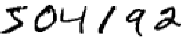
Easy right? — Most people effortlessly recognize those digits as 504192. That ease is deceptive. You didn’t even bother about the poor resolution of the image, how amazing. We should all take a moment to thank our brains! Wonder how natural it is for our brains to process the image, classify it and respond back. We are gifted!

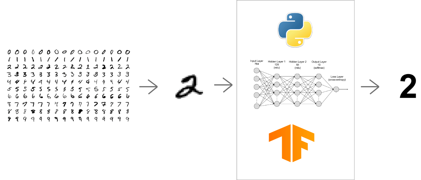
How difficult would it be to imitate the human brain? Deep learning, in easy terms, is the area of machine learning research, which allows the computer to learn to perform tasks which are natural for the brain like handwritten digit recognition.

In this article, we will be discussing neural networks and along the way will develop a handwritten digit classifier from scratch. We will be using Tensorflow because it is cool!

The only prerequisite to this article is basic knowledge about Python syntax .

Knowing The Dataset :

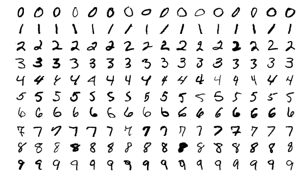
The most crucial task as a Data Scientist is to gather the perfect dataset and to understand it thoroughly. Trust me, the rest is a lot easier. For this project, we will be using the popular MNIST database. It is a collection of 70000 handwritten digits split into training and test set of 60000 and 10000 images respectively.

To begin our journey with Tensorflow, we will be using the MNIST database to create an image identifying model based on simple feedforward neural network with no hidden layers.

MNIST is a computer vision database consisting of handwritten digits, with labels identifying the digits. As mentioned earlier, every MNIST data point has two parts: an image of a handwritten digit and a corresponding label.

We’ll call the images “x” and the labels “y” . Both the training set and test set contain images and their corresponding labels; for example, the training images are mnist.train.images and the training labels are mnist.train.labels.

Each image is 28 pixels by 28 pixels. We can interpret this as a big array of numbers. We can flatten this array into a vector of 28×28 = 784 numbers.

It doesn’t matter how we flatten the array, as long as we’re consistent between images. From this perspective, the MNIST images are just a bunch of points in a 784 -dimentional vector space.

To begin our journey with Tensorflow, we will be using the MNIST database to create an image identifying model based on simple feedforward neural network with no hidden layers.

MNIST is a computer vision database consisting of handwritten digits, with labels identifying the digits. As mentioned earlier, every MNIST data point has two parts: an image of a handwritten digit and a corresponding label.

We’ll call the images “x” and the labels “y”. Both the training set and test set contain images and their corresponding labels; for example, the training images are mnist.train.images and the training labels are mnist.train.labels.

Each image is 28 pixels by 28 pixels. We can interpret this as a big array of numbers. We can flatten this array into a vector of 28×28 = 784 numbers.

It doesn’t matter how we flatten the array, as long as we’re consistent between images. From this perspective, the MNIST images are just a bunch of points in a 784 -dimentional vector space.

To begin our journey with Tensorflow, we will be using the MNIST database to create an image identifying model based on simple feedforward neural network with no hidden layers.

MNIST is a computer vision database consisting of handwritten digits, with labels identifying the digits. As mentioned earlier, every MNIST data point has two parts: an image of a handwritten digit and a corresponding label.

We’ll call the images “x” and the labels “y”. Both the training set and test set contain images and their corresponding labels; for example, the training images are mnist.train.images and the training labels are mnist.train.labels.

Each image is 28 pixels by 28 pixels. We can interpret this as a big array of numbers. We can flatten this array into a vector of 28×28 = 784 numbers.

Download the MNIST

from tensorflow.examples.tutorials.mnist import input_data

mnist= input_data.read_data_sets(“model_data/", one_hot=True)

Import Tensorflow to your environment

import tensorflow as tf

Initializing parameters for the model

batch =100

learning_rate=0.01

training_epochs=10

In machine learning, an epoch is a full iteration over samples. Here, we are restricting the model to 10 complete epochs or cycles of the algorithm running through the dataset.

The batch variable determines the amount of data being fed to the algorithm at any given time, in this case, 100 images.

The learning rate controls the size of the parameters and rates, thereby affecting the rate at which the model “learns”.

Creating Placeholders

x=tf.placeholder(tf.float32, shape=[None, 784])

y=tf.placeholder(tf.float32, shape=[None, 10])

The method tf.placeholder allows us to create variables that act as nodes holding the data. Here, x is a 2-dimensionall array holding the MNIST images, with none implying the batch size (which can be of any size) and 784 being a single 28×28 image. y_ is the target output class that consists of a 2-dimensional array of 10 classes (denoting the numbers 0-9) that identify what digit is stored in each image.

Creating Variables

W = tf.Variable(tf.zeros([784, 10]))

b=tf.Variable(tf.zeros([10]))

Here, W is the weight and b is the bias of the model. They are initialized with tf.Variable as they are components of the computational graph that need to change values with the input of each different neuron.

Initializing the model

y=tf.nn.softmax(tf.matmul(x,W) + b)

We will be using a simple softmax model to implement our network. Softmax is a generalization of logistic regression, usually used in the final layer of a network. It is useful because it helps in multi-classification models where a given output can be a list of many different things.

It provides values between 0 to 1 that in addition give you the probability of the output belonging to a particular class.

Defining Cost Function

cross_entropy
=tf.reduce_mean (tf.reduce_sum(y_*tf.log(y),
reduction_indices=[1]))

This is the cost function of the model–a cost function is a difference between the predicted value and the actual value that we are trying to minimize to improve the accuracy of the model.

Determining the accuracy of parameters

correct_prediction= tf.equal(tf.argmax(y,1),tf.argmax(y_,1))

accuracy= tf.reduce_mean
(tf.cast(correct_prediction,tf.float32)

Implementing Gradient Descent Algorithm

with tf.Session() as sess:

sess.run(tf.initialize_all_variables())

Creating batches of data for epochs

for epoch in range(training_epochs):

batch_count= int(mnist.train.num_examples/batch)

for i in range(batch_count):

batch_x,batch_y= mnist.train.next_batch(batch)

Executing the model

sess.run([train_op],feed_dict={x:batch_x, y_:batch_y})

Print accuracy of the model

if epoch%2==0:

print "Epoch: ",epoch

print "Accuracy: ", accuracy.eval(feed_dict={x: mnist.test.images, y_: mnist.test.labels})

print "Model Execution Complete"

Share your accuracy details I would love to see those